PCA and Face Recognition - Eigen Face
PCA (Principal component analysis), just as its name shows, it computes the data set’s internal structure, its “principal components”.
Considering a set of 2 dimensional data, for one data point, it has 2 dimensions \(x_1\) and \(x_2\) . Now we get n such data points . What is the relationship between the first dimension \(x_1\) and the second dimension \(x_2\) ? We compute the so called covariance:
\[cov(x_1,x_2)=\frac{\displaystyle \sum_{i=1}^n{(x_1^i-\overline{x_1})(x_2^i-\overline{x_2})} }{n-1}\]the covariance shows how strong is the relationship between \(x_1\) and \(x_2\). Its logic is the same as Chebyshev’s sum inequality:
\(a_1>a_2>. . . >a_n \\ and\\ b_1>b_2>. . . >b_n \\ then\\ \frac{1}{n}\displaystyle \sum_{k=1}^n{a_k\cdot b_k}\geq(\frac{1}{n}\displaystyle \sum_{k=1}^na_k)(\frac{1}{n}\displaystyle \sum_{k=1}^nb_k)\)
Which tells us a truth:
big with big, small with small can result big value;big with small, small with big can result small value.
So on the other way around, \(cov(x_1,x_2)\) measures how the data points’ \(x_1\) and \(x_2\) are related to each other, let’s say data point \(P:(x_1^p,x_2^p)\) , if \(x_1^p-\overline{x_1}\) is relatively big compared to the other \(x_1s\) and the same for \(x_2^p\), then \((x_1^p-\overline{x_1})(x_2^p-\overline{x_2})\) will be big, which will be added to the final \(cov\) value, if \(x_1\) and \(x_2\) changes in the same direction, which means when \(x_1\) gets big, \(x_2\) also gets big, the \(cov\) value will be very big. The changing direction of both dimensions are more different to each other, the smaller is the final \(cov\) value.
We compute \(cov(x_1,x_2)\),\(cov(x_1,x_1)\) and \(cov(x_2,x_2)\), obviously \(cov(x_2,x_1)\) will be the same as \(cov(x_1,x_2)\). These 3 values will form a matrix, the so called covariance matrix:
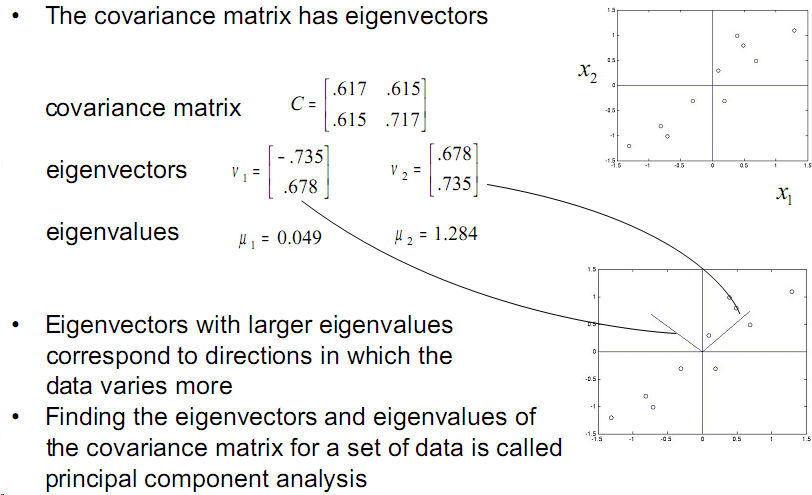
the dots in the upper right chart means one data point \((x_1^i,x_2^i)\)
The C matrix is the covariance matrix, lower are its eigen vector and eigen value.
As we can see from the eigen vector’s visualization, if the point dots can form a ellipse, the eigen vectors will be its long and short axis. The corresponding eigen values are their lengths.
Use PCA to recognize faces
Our input:the image of a face
Our training set: face images of different people
Out output: who is this input face?
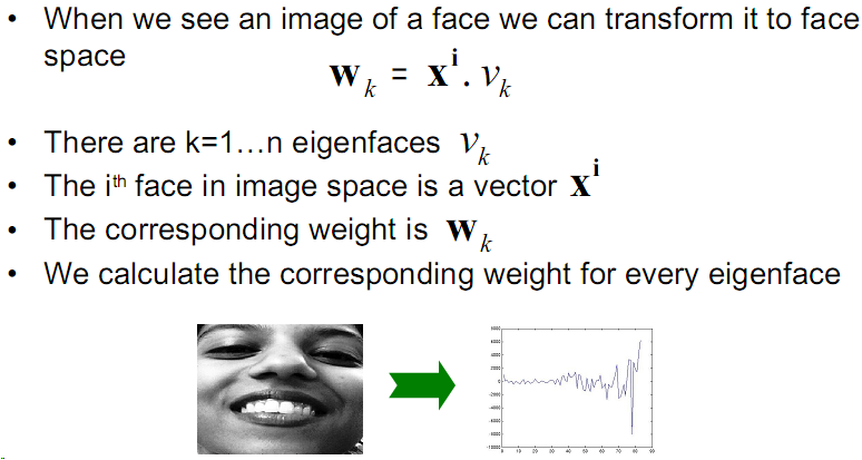
We consider a face image is a point in high-dimensional space.
The training set of face images will be our point set, just as one dot in the upper chart. Remember, this face image data set only contains the face images of one person.
Training:
The training process will be calculating this data set’s covariance matrix and its eigen vectors and eigen values.For this task we use SVD, assume that we have the data matrix X, after the SVD we get:
\[X=U\Sigma V^*\]What we want is the eigenvalues and eigenvectors of X’s covariance matrix:\(XX^T\)
According to the properties of SVD, we get:
\[XX^T=U\Sigma^2U^T\\\]As we know that \(U\) is an orthogonal matrix, which means \(U^T=U^{-1}\) , so we get:
\[XX^TU=U\Sigma^2\]Obviously, The vectors in U are the eigenvectors of \(XX^T\) and the square of the values in \(\Sigma\) are its eigenvalues.
Practically:
For a image of 100x100, we get a data point in a 10000 dimensional space. Then we can calculate a 10000x10000 covariance matrix. From this matrix we get a 10000 dimensional eigen vector whose eigen value is the biggest of all eigen values.
This 10000 eigen vector is of course also a face image, it is the so called eigen face or basis face. Eigen face is the computed face image which contains the most important features of this person.
Matching/Recognition: