Discriminatively Trained Part Based Models notes

The LSVM (SVM with latent variable) is mostly used for human figure detection, it is very efficiency because it puts the human figure’s structure into consideration: a human figure has hands, head and legs. The LSVM models the human figure structure with 6 parts, and the position of these 6 parts are latent value.

The basic logic is sliding a window on the image, for every position we get a small image patch, by scoring this image patch we can predict whether this image patch contains a human figure or not.

Defining the score function

Anyway, the first thing to do: defining a score function:

Assumptions: we already trained the model and now we are using this model to find the image patch which contains a human figure by computing the score.

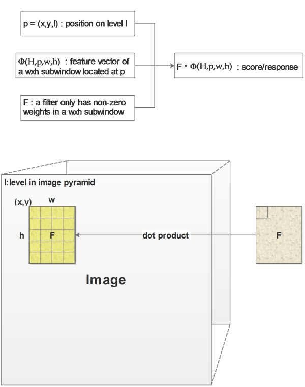
Just as a normal sliding window method, we search the whole image pyramid, so the position \(p\) of a image patch will be defined by x, y and l. l short for “level” represents the level in a image pyramid.

We are evaluating a image patch, instead of directly using its pixel values, we will use the feature vector computed from this image patch, \(\Phi(H,p,w,h)\) is the feature vector extracted from the image I.

\(H\) is short for HoG feature, as we are using HoG feature , more precisely, \(H\) is the pyramid of HoG features computed from I.

p is the position of the upper left corner of the current image patch

w and h are the width and height of the image patch.

\(F\) will be the weights vector, in this paper it is called filter, because it is represented by a weighted window filter which only has none-zero weights at the position of image patch.

Finally we get the score by computing the dot product of \(F\) and \(\Phi\):

Remember that we consider a human figure to be a structured model with 6 separate parts, let’s visualize it in the following image:

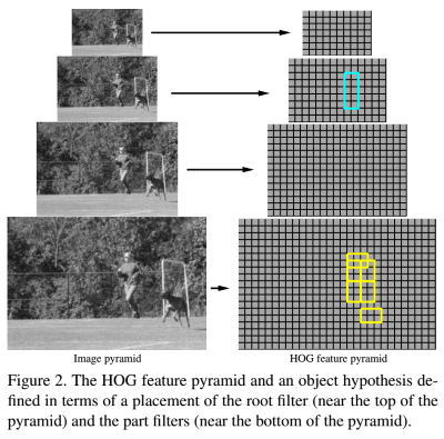
Our model has a root filter highlighted as cyan rectangle, this root filter is used to find the whole human figure as a rough prediction. It will be computed in the feature pyramid’s high level to locate the human.

Apart from the root filter, we have the other 6 part filters highlighted as yellow rectangles in the above image. These filters will be positioned with some flexibility relative to the root filter, each filter of cause provide their own scores, the following diagram shows how are all these scores combined together to form a final score:

\(F_0\) is the root filter, \(P_1 . . . P_n\) are the part filters and \(b\) is the bias.

For one part filter \(P_i\):

​ \(F_i\) is its filter

​ \(v_i\) is the anchor of the filter, the position of where it should be:

​ - it is learned from the learning process.

​ \(d_i\) is the parameters used to compute the penalty of the ith part:

​ - The part filter should not be too far away from where it should be

​ - The final score will be penalized by the position of the ith filter:

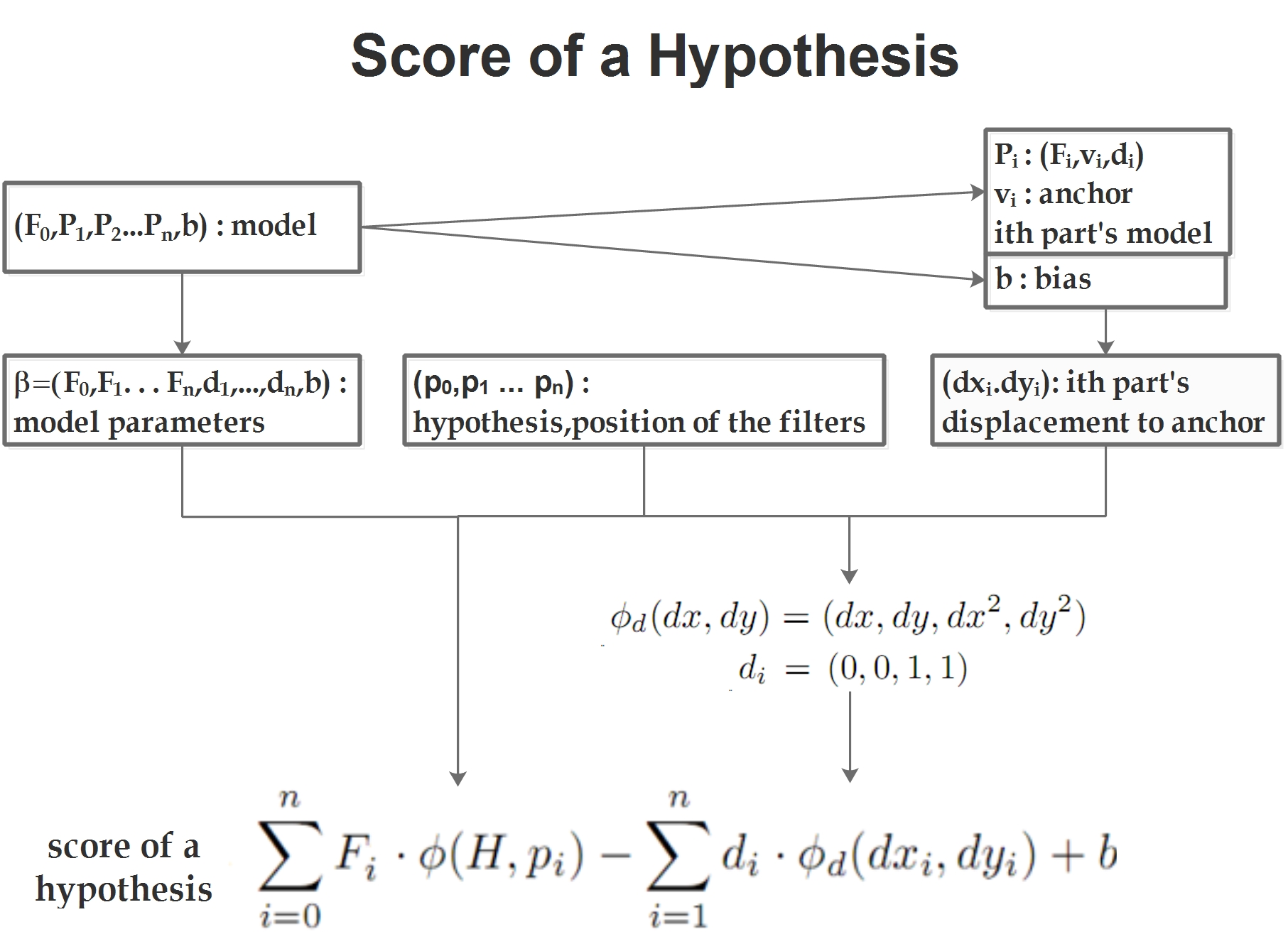
So the score of a complete model is a summation of:

the scores of the root and part filters and

the penalty of the part filters’ position.

Matching

Now we have the function to score a hypothesis image patch, as we can see, there are some variables which are unclear:

How can we find the location of the root filter?

That’s easy, we are simply sliding the foot filter in the whole image pyramid, defining its position only by computing the root filter’s score

How can we find the location of the part filters?

Once we find the location of the root filter, we can say it is very possible that there is a human figure in the image patch covered by the filter.

Then we can further position the part filters and compute the final score to evaluate if this image patch is really a human figure.

Positioning the part filters allows some flexibility, that’s why it’s called “latent”:

again, the ith part filter at position \(x,y,l\):

\[R_{i,l}(x,y)=F_i\cdot\phi(H,(x,y,l))\]

The latent part: position of the ith filter is latent, move it around to find the best position:

\[D_{i,l}(x,y)=max_{dx,dy}(R_{i,l}(x+dx,y=dy)-d_i\cdot\phi_d(dx,dy))\]

so adding the score of the root filter, we get the final score:

\[\displaystyle R_{0,l_0}(x_0.y_0)+\sum_{i=1}^nD_{i,l_0-\lambda}(2(x_0,y_0)+v_i)+b\]

So the matching process can be described as:

1. sliding the root filter to find the root position

2. sliding the 1st part filter around its anchor position(learned in the training) relative to the root position until this part filter gets the max score, fix it.

3. sliding the 2nd, 3rd …. until all part filters are fixed

4. sum all the scores of root and part filters and the penalty part

When we find a postion with a score bigger than the threshold, we can say we find a human figure image patch.

One more thing to add: making the position of the root filter latent can help to improve the result.

Training

The left part:

The left part of the diagram shows a normal SVM problem using the Hinge Loss function to achieve the optimization goal \(L_D(\beta)\).

We have a training image set with a series of images \(x\) labeled with their class \(y\), in this case, if the image \(x\) is human figure, we label it as 1, if it doesn’t contain a human figure, it will be labelled -1.

\(D\) is short for “data set”, which contains all the sample images.

\(\beta\) is the model parameter vector which is our training target, the weights.

\(\phi\) is the feature vector

\(z\) are the latent values to locate the part filters

Just as the normal gradient descent algorithm, we differentiate \(L_D(\beta)\) according to \(\beta\) , with the step length \(\alpha_t\) , \(t\) is the current iteration.

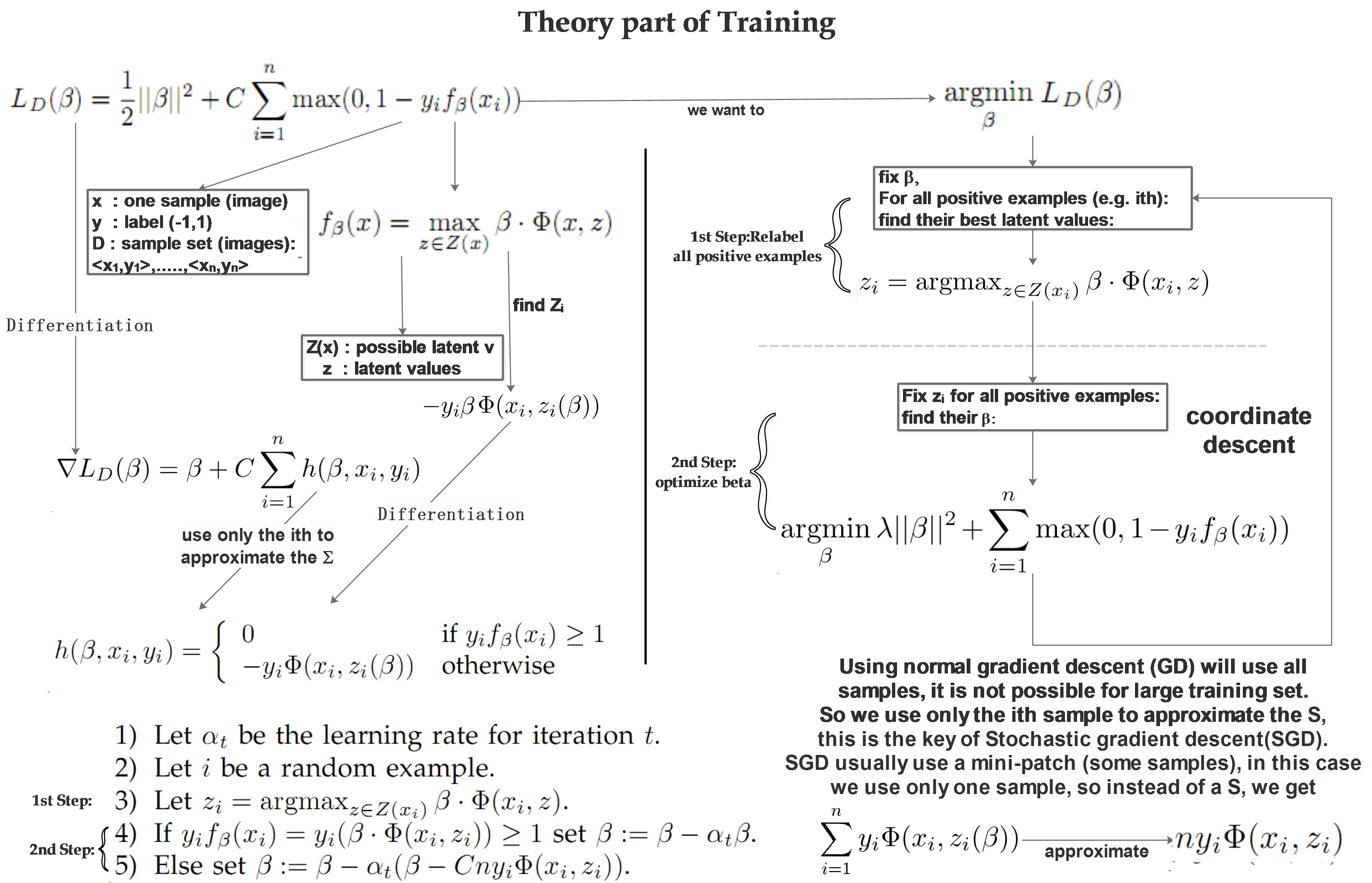
The right part:

The right part of the diagram shows how the learning process is done.

The learning process has 2 steps:

In the 1st step, we fix \(\beta\) and search in the whole image to locate the part filters’ positions (find the latent variables). As we are now learning, so we know that this image contains a human figure, then we don’t need to care about the root filter, or we can say, the root filter’s position is (0,0).

In the 2nd step, we fix the latent variables and update \(\beta\) .

Training in practice

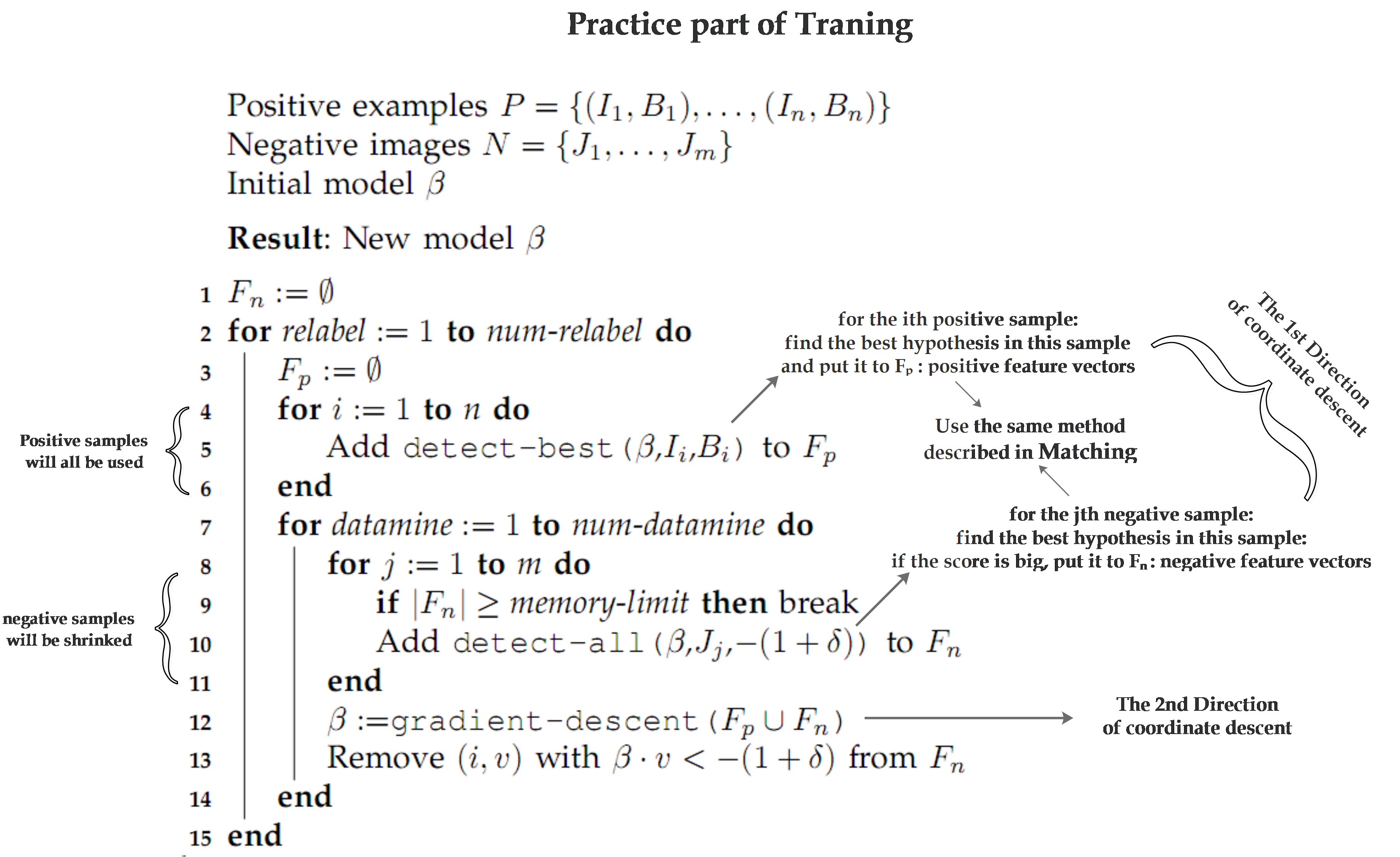
Initialization: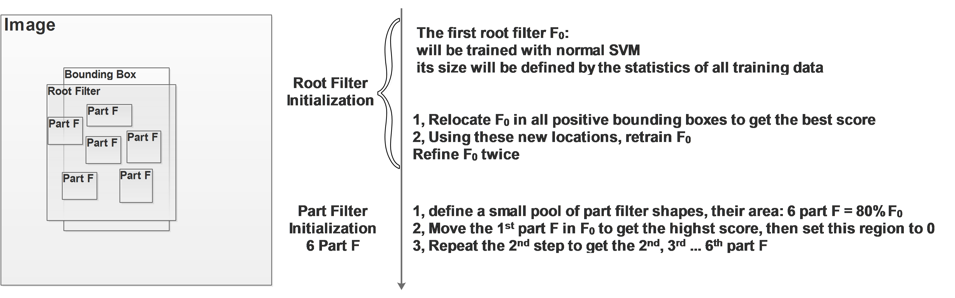

Appendix:

How to solve the optimization problem?

For an input pair \({x_i,y_i}\)，we get a prediction from ω：\(f_ω (x_i)\)

Using the normal hinge loss function as the loss function, we get the following optimization problem:

\[\displaystyle argmin_ω{\left\{ \frac{1}{2}|ω|^2 +C\sum_{i=1}^Nmax(0,1-y_i\cdot f_\omega(x_i)) \right\} }\]

as a normal SVM problem, it’s easy to solve.

But in this case, we introduce the latent value h，\(f_ω (x_i)\) is no longer a easy linear function like \(ω\cdot x_i+b\).

It is now：

\[f_ω (x_i )=\max_{h\inΗ}⁡ω\cdotΦ(x_i,h)\]

Which means，prediction turns to be a discrete non-linear function related to latent value, which cause the above problem difficult to solve.

But you will find out that \(h\) and \(\omega\) are independent to each other, so we can treat them as two independent variables, then we can use coordinate descent algorithm to solve this optimization problem.

The first step, fix \(\omega\), update \(h_i:h_1\cdots h_N\)

Which means, assuming that we know \(\omega\) already, we compute a \(h_i\) using:

\[f_ω (x_i )=\max_{h\inΗ}⁡ω\cdotΦ(x_i,h)\]

now we fix \(h_i\), \(f_ω (x_i)\) then turns to be a normal convex linear function to \(\omega\).

The second step, fix \(h_i:h_1\cdots h_N\), update \(\omega\):

So for each \(i\), after we computed the \(h_i\) based on the already existed \(\omega\), \(\max⁡(0,1−y_if_ω (x_i))\) turns to be a convex function.

And we know that the summation of convex functions will be still convex.

So we can find the sum of all \(max⁡(0,1−y_if_ω (x_i))\) for \(i=1\cdots N\), the summation will be still convex.

Original Paper :

A Discriminatively Trained, Multiscale, Deformable Part Model

Object Detection with Discriminatively Trained Part Based Model