Linear Classification

Loss Function

Now we want to solve a image classification problem, for example classifying an image to be cow or cat. The machine learning algorithm will score a unclassified image according to different classes, and decide which class does this image belong to based on the score. One of the keys of the classification algorithm is designing this loss function.

Map/compute image pixels to the confidence score of each class

Assume a training set:

\[(x_i,y_i)\]

\(x_i\) is the image and \(y_i\) is the corresponding class

i∈1…N means the traning set constains N images

\(y_i\)∈1…K means there are K image categories

So a score function maps x to y:

\[f(x_i,W,b)=W\cdot x_i+b\]

In the above function, each image \(x_i\) is flattend to a 1 dimention vector

If one image’s size is 32x32 pixels with 3 channels

\(x_i\) will be a 1 dimention vector with the length of D=32x32x3=3072 Parameter matrix W has the size of [KxD], it is often called weights b of size [Kx1] is often called bias vector In this way, W is evaluating \(x_i\)’s confidence score for K categories at the same time

The physical meaning of loss function

W uses weights to decide the importance of each pixel，for example a W used to classify a ship，its weights for blue channel on the pixels located on the image border will be big, cause normally a ship in an image is surrounded by blue sea.

The geometrical meaning of loss function

Considering an image \(x_i\) to be a point in a hyperspace，then obviously W and b， forms a hyper-plane in this space, b will the intercept and W will be the slop，if we substitute the loss function with \(x_i\) and get a positive value，it means \(x_i\) is “under” the hyper-plane, or it’s under the plane.

How loos function looks like, visually?

The learned W matrix contains the information of its corresponding image class, to be exact, the W of an image class can also be considered as an image, whose pixels are its weight values, and the weights mean the most probable RGB values. So obviously, W as an image looks like the image of its corresponding class, roughly:

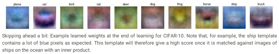
In the above images, the W of “horse” images shows a horse with two heads, that’s because the learning result merges the images with the horses fronting left and right.

The weight image of the class “car” is red, it means there are too many red cars in our training set.

All these factors cause the inaccuracy and lower generalization ability.

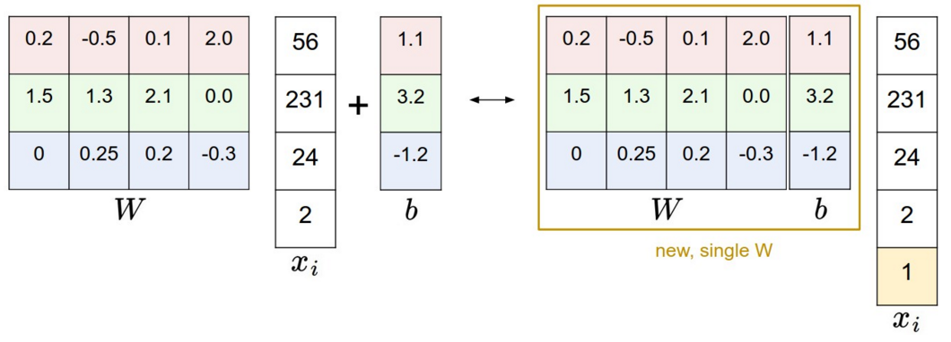
Usually we put the intercept \(b\) into \(W\) and on the other side add one dimension into \(x_i\) and fill it with all 1, then:

\[f(x_i,W,b)=W\cdot x_i+b\]

turns to

\[f(x_i,W)=W\cdot x_i\]

just as the following diagram shows:

Preprocessing to the original data

For the input images, we can not use the original image, they should be normalized.

Firstly we compute the average image of all images in the training set and subtract it from all the images (centering), after that (now the pixel values should be -127~127) we scale the values further to \([-1,1]\).

Hinge Loss function

Hinge loss function computes the difference of the two scores: the score when an image is classified correctly and the score when it’s classified wrongly.

For example, for the \(i\)th sample in the training set \((x_i,y_i)\):

\[L_i= \sum_{j≠y_i}max(0,w_j^T\cdot x_i−w_{y_i}^T\cdot x_i+Δ)\]

\(w_j^T\cdot x_i\) is the score classifying \(x_i\) to class \(j\)，and \(w_{y_i}^T\cdot x_i\) is the score when it’s classified correctly(classify to class \(y_i\))，\(\omega_i\) is the \(j\)th row in \(W\).

Normally, the score is positive when classified correctly and it’s very big. When it’s classified wrongly(classified to \(j\), wrong), the score will be negative.

In this case, if we subtract the score of correct classification from the score of wrong classification we get a very small negative value, so \(L_i\) will be \(0\), which means no loss.

Sometimes, the score of correct classification of a sample image is relatively small, even negative, and it may be even positive when classified to class \(j\).

In this case, if we subtract the score of correct classification from the score of wrong classification we get a positive value. Which means the loss is very big.

Then what is \(\Delta\) ? Let’s take a look at the following diagram:

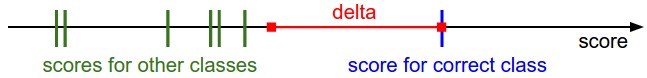
When \(\Delta\) is 0, we define the loss based on the score’s absolute value, this condition is too loose, because if the score of correct classification is just a little bit bigger than the wrong classification, we still get \(0\) loss, actually this case is very confusing.

So \(\Delta\) is actually a confidential interval, which means, it is not enough that the score of correct classification is bigger then the wrong classification, their difference must be bigger than \(\Delta\). On the other hand, if both scores have only little difference, the loss will be at least \(\Delta\).