Graph Optimization 4 - g2o introduction - GPS odometry
In graph optimization 1 to 3, the math is introduced. Now we can make some hands on practice on programming. The most famous used graph optimization library is g2o due to its good performance in ORB-SLAM. g2o also has its well known drawback - not well commented, not easy to understand. What’s more, most of the tutorials are based on the original sample examples, when you want to make your own vertex or edge, you will again be lost.
This introduction will be based on an easy to understand graph optimization problem with a customized edge implementation.
Modelling the GPS based odometry
Model as graph
The problem is quite easy: we have a vehicle moving around, we use a GPS to measure its 3D absolute positions, by making some rough guesses as initialization, we want to estimate the vehicle’s position based on the GPS’ measurements.
In a SLAM system, we usually want to fuse different sensors, what’s discussed most are fusing camera and IMU, which is also the problem setup for g2o examples. Fusing GPS information is rarely touched, actually GPS sensor fusion is easier to understand. It can be modeled as the following diagram:
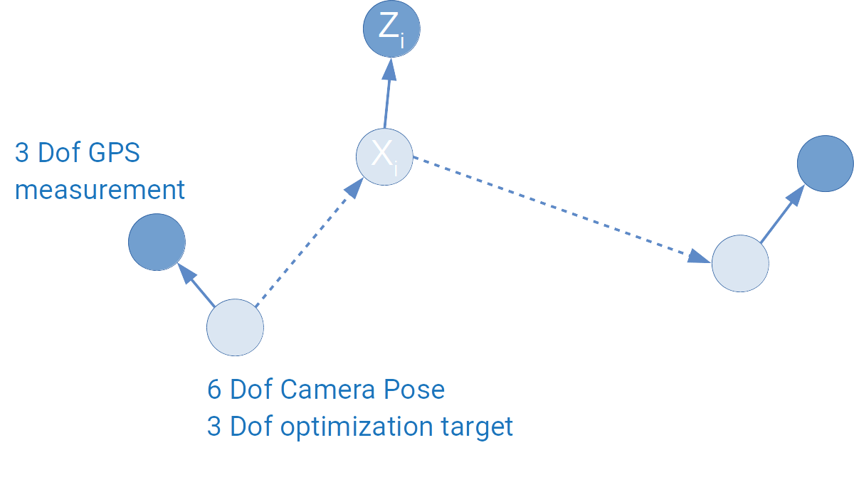
The light blue vertexes are camera poses to be estimated, it’s represented as 6 Dof pose just for the convenience of future work, considering only GPS measurements, only 3 Dof will be optimized.
The dark blue vertexes are GPS measurements, they are fixed. The dark blue arrows are the edges representing the error between the measurement and estimation, which in our case is simply the difference between the measurement and the estimation.
The dark blue vertexes are “pulling” the light blue vertexes toward them, just as what’s happening in the real world : we try to estimate something that fit the measurements best.
Model as equation
The optimization problem can be expressed as the following equation:
\[X^*_{1..i}=\arg \max_{X_{1..i}}\sum_i(e_{i}^T\Omega_i e_i)\]\(X_i\) is the estimation, which is being updated in the optimization loop; \(Z_i\) is the measurement for \(X_i\) , which is fixed; the error \(e_i\) is the error we get between estimation and measurement.
\(\Omega\) is the so called “information” matrix, in our case, as the poses are not correlated to each other, it is a identical matrix, if we consider \(\Omega_i\) is its \(i\)th diagonal element, \(\Omega_i\) will always be one.
Put the error in, we get the complete equation:
\[X^*_{1..i}=\arg \max_{X_{1..i}}\sum_i((X_i-Z_i)^T\Omega_i (X_i-Z_i))\]For the graph optimization problem, we also need the Jacobian matrix, which contains:
\[\frac{d e_i}{d X_i}=\frac{d(X_i-Z_i)}{d X_i}=1\]Obviously, our Jacobian matrix is also a diagonal matrix!
Now, we get everything ready for the math.
Solving the problem with g2o
How is g2o structured?
Define Optimizer
The core of g2o is based on the Optimizer, which can be considered as the optimization engine managing everything. As the optimization problem in the field of SLAM is mostly sparse, we usually use the sparse optimizer. The sparse optimizer will take the sparsity of the Jacobian matrix into consideration and saves time and space. So the first step of our program will be declaring an optimizer:
g2o::SparseOptimizer optimizer;
Define Optimization algorithm
From Graph Optimization 3 we get the update equation:
\[H(x_0)\Delta x^*=-b(x_0)\]In order to compute \(\Delta x^*\) , we need to compute \(H(x_0)^{-1}\). If the parameter space is large, the \(H\) matrix will be also large and computing the inverse will be really heavy. Just as mentioned above, the \(H\) matrix is usually a sparse matrix, if we know its structure in beforehand, we can “densify” it and solve its inverse to save time and space, which is the so called “Schur complement”. When the \(H\) matrix is “densified”, we can also use different methods to solve its inverse.
When the structure of the \(H\) matrix and the method of computing matrix inverse is defined, we can finally define the solver type. g2o is a perfectly designed object oriented library, it can define the solver type in one line combining all these information:
auto linearSolverType = g2o::make_unique<g2o::LinearSolverCholmod <g2o::BlockSolverPL<6,1>::PoseMatrixType>>();
When the solver type is defined, we can then create a solver:
auto solver = g2o::make_unique<g2o::BlockSolverPL<6, 1>>(std::move(linearSolverType));
With the newly created solver, we can finally create the optimization algorithm:
g2o::OptimizationAlgorithmLevenberg* optimaAlgorithm = new g2o::OptimizationAlgorithmLevenberg(std::move(solver));
The above 3 lines of code are obviously not friendly at all, I will explain them further in detail.
Optimization Algorithm
Many algorithms can be used for optimization, such as Gauss-Newton, Gradient-Descent , Levenberg-Marquardt and so on. Here we use Levenberg-Marquardt algorithm to optimize the problem. In g2o it is implemented as a class “g2o::OptimizationAlgorithmLevenberg”.
Solver Type
auto linearSolverType = g2o::make_unique<g2o::LinearSolverCholmod g2o::BlockSolverPL<6,1::PoseMatrixType>>();
The solver type defines the method to solve the matrix inverse and the structure of the sparse matrix. Firstly we are solving a \(Ax=b\) problem, then the solver is called “LinearSolver”, as we use Cholmod as the back-end library to solve this linear problem, we define the solver type as LinearSolverCholmod. There is also a solver type class LinearSolverCsparse which us Csparse library as the back end solver.
When solving a sparse matrix, we treat the matrix as blocks to do the Schur Complement. In order to treat it correctly, we need to specify how is the matrix structured. For our GPS odometry problem, we optimize the 6 Dof camera pose, therefore the block size of the matrix will be 6x1, the matrix type will be g2o::BlockSolverPL<6,1>::PoseMatrixType. Actually only 3 Dof can be optimized based on the GPS constraint, as we want to fuse other odometry information later, we define the camera pose to be 6 Dof.
Solver
auto solver = g2o::make_unique<g2o::BlockSolverPL<6, 1>>(std::move(linearSolverType));
BlockSolverPL is a template of the BlockSolver which supports user-defined block size. Here we create a solver for computing the inverse of matrix \(H\).
With the solver, we then create a optimization algorithm engine:
g2o::OptimizationAlgorithmLevenberg* optimaAlgorithm = new g2o::OptimizationAlgorithmLevenberg(std::move(solver));
unique pointer and move
From the very beginning, we use unique pointer and move function to create new instances. The input solver of the optimization algorithm engine’s constructor is asked to be an unique pointer, which can guarantee that the pointer of solver will only be accessed by the optimization algorithm and make sure the solver is thread safe. We can see move function everywhere as the unique pointers can only moved, there is no way to get access to a unique pointer at the same time in two threads.
Run the optimizer
When the optimization algorithm is fully defined and created, it can then be used to setup the optimizer:
optimizer.setAlgorithm(optimaAlgorithm);
After this step, we can model the optimization problem by adding vertexes and edges into the optimizer, this part will be explained in the following article.
Once we setup the graph model, we can call the following two functions to initialize and run the optimizer:
optimizer.initializeOptimization();
optimizer.optimize(100);
The optimizer will run at most 100 iterations according to the settings above. If we want to observe the optimization process, we can call
optimizer.setVerbose(false);
to print out the intermediate information.