NN Preprocessing

Centering and Scaling

Some preprocessing is needed before the training.

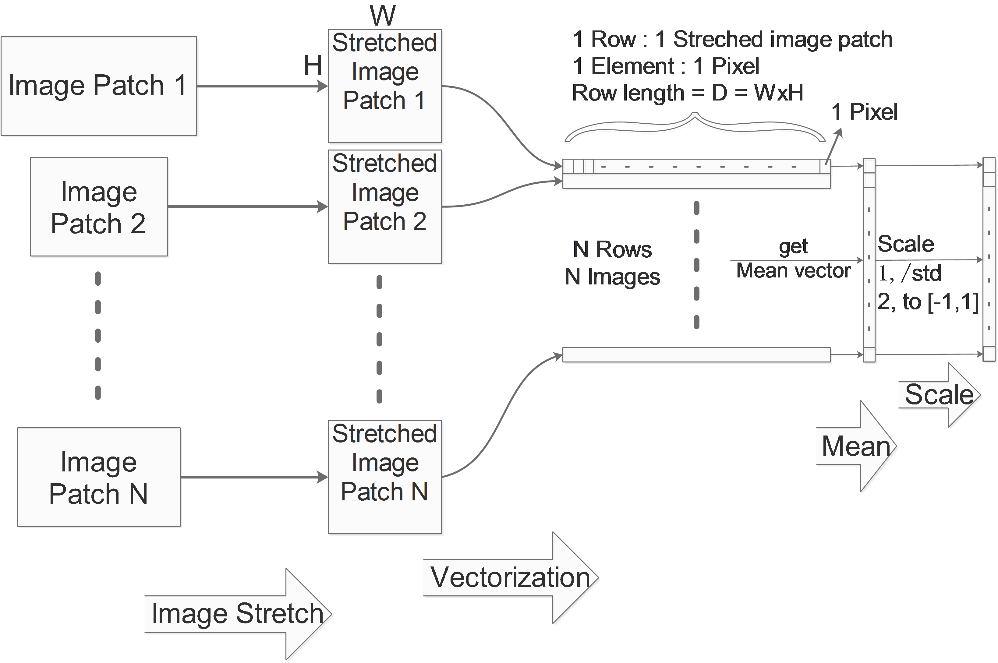
Image Stretch

If we are dealing with images and the image patches in the data set have different sizes, then the data can not be aligned. So we need to firstly stretch all the image patches to the same size.

Image Vectorization

One image in the dataset will be vectorized to one vector as a row. Considering a gray image with the size of WxH, its corresponding row vector’s size will be D=W*H.

We collect these rows in one big matrix, for a N images data set, we get a NxD matrix which contains all information of the whole data set. We call it X.

Data Centering

Each data row of the data matrix X should be centered, we compute the mean value for each data row and subtract the mean value pixel by pixel from this data row. Each data row will be centered independently, after the centering process, the mean value of each data row will be 0.

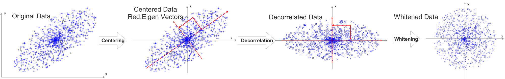
Taking a 2D data set as an example, the centering process can be visualized as:

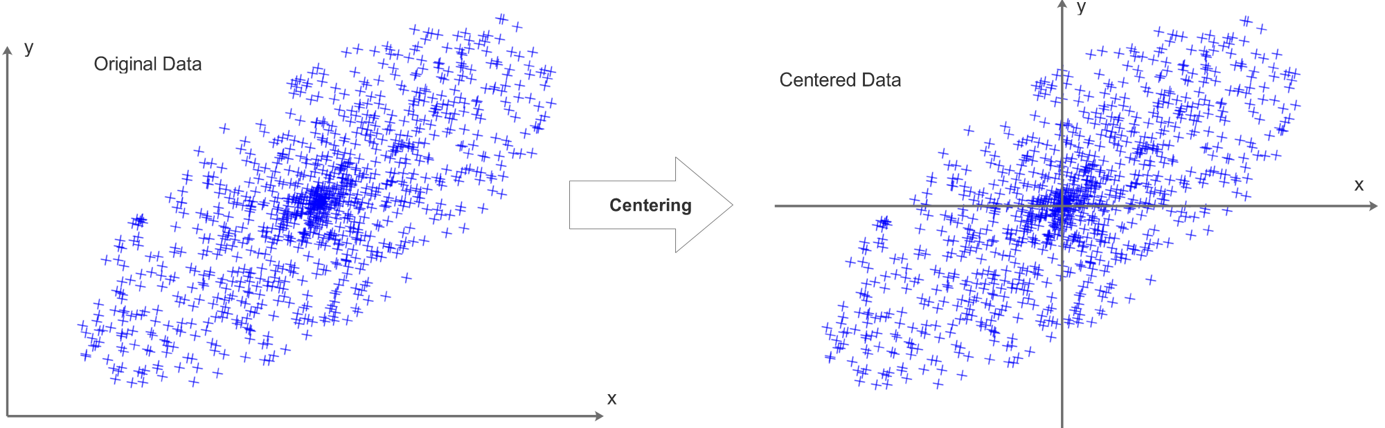
It is also common to compute the means of all data and get one single mean value. This mean value will then be subtracted from all pixels/data elements.

Data Normalization

The data will then be normalized, the process can be visualized as:

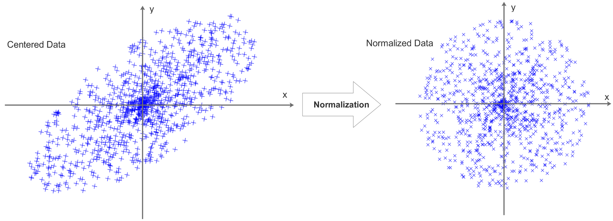
Now we can see that centering data is actually a preparation for normalization, decentered data can not be normalized. There are 2 ways to normalize the data:

1, Compute the standard deviation of each data row and divide each pixel by the STD of its data row.

2, Scale each data row to [-1,1]

Data Decorrelation

Before normalization, decorrelation is required, it can be visualized as:

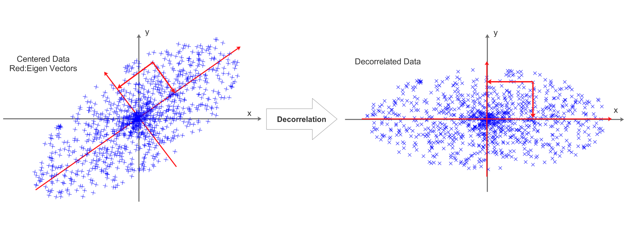
This process is achieved by PCA:

We firstly compute the covariance matrix of X ( Normalize( Center(X) ) ):

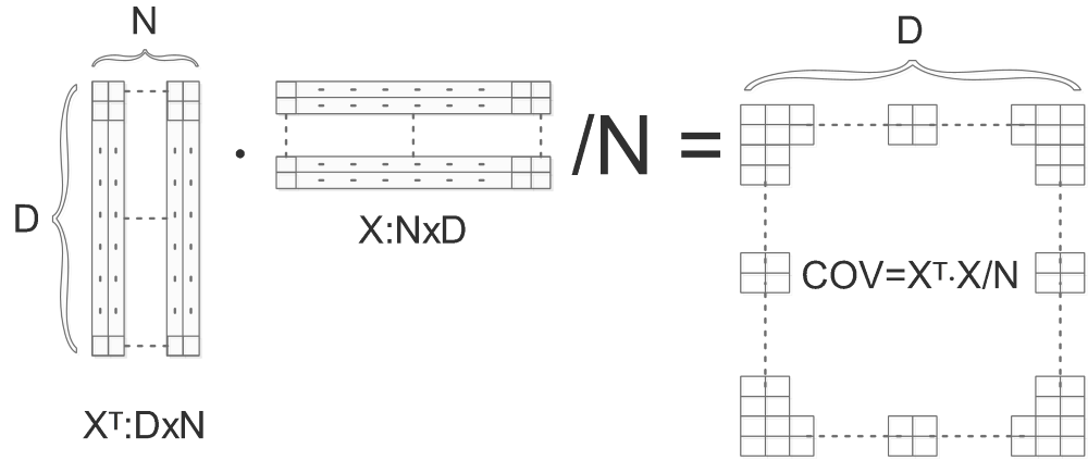
COV is the computed covariance matrix, we do SVD on COV and get U,S,V:

\[[U,S,V]=svd(COV)\]

The columns of U are eigen vectors and the diagonal values of S are singular values. Eigen vectors are orthonormal with the length of D, they can be considered as bases.

Actually, we can also do SVD directly on X:

\[[u,s,v]=svd(X)\]

Comparing \(U,S,V\) and \(u,s,v\):

\(v\) is exactly the same as \(U\).

\(u\) is exactly the same as \(V\).

The eigen vectors are visualized as red vectors in the above diagram.

We can “project” the data point on to the eigen vectors:

\[RotX=Decorrelated(X)=X\cdot U=X\cdot v\]

The projection is visualized as the 2 projection arrows perpendicular to each other. After the projection, the decorrelated data’s eigen vectors will be aligned with x and y axis.

Dimensionality Reduction

The eigen vectors in \(U\) are already sorted by the singular values in \(S\), the bigger is the singular value, the more important is the corresponding eigen vector in \(U\)：

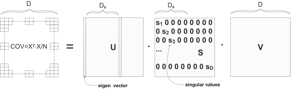
In the above diagram, the singular values are already sorted from big to small:

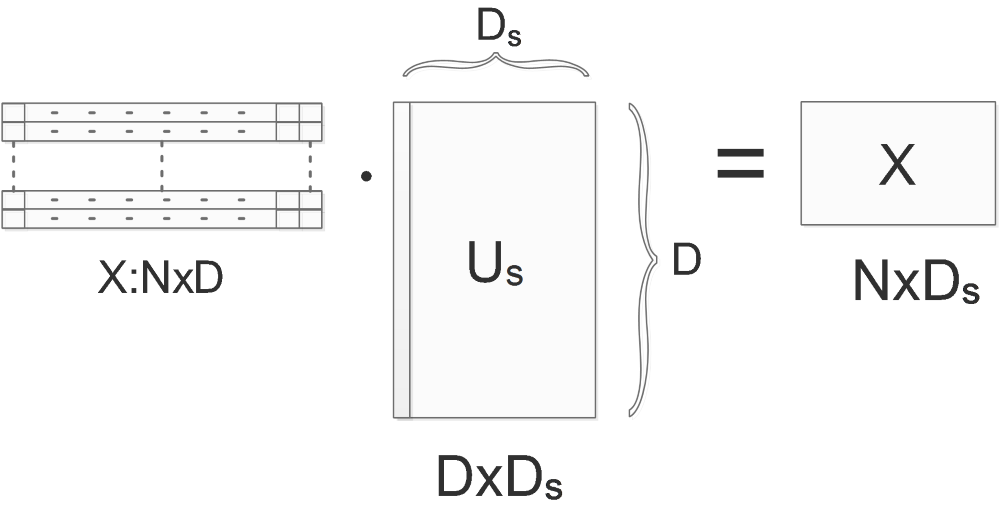
\[s_1>s_2>\cdots >s_N\]

So we can ignore the less important eigen vectors. Let’s say the first \(D_s\) singular values are big enough to be kept. So we use only the first \(D_s\) columns of \(U\) to project the original data:

Normally, when decorrelatting the \(X\), we use the whole \(U\) matrix(the \(v\)) to project:

\[RotX=Decorrelated(X)=X\cdot U=X\cdot v\]

Now we throw the less important directions(eigenbases) away, the data will then be projected to the first \(D_s\) directions:

\[RedRotX=Reduced\_Decorrelated(X)=X\cdot U_s=X\cdot v_s\]

The size of \(RotX\) is originally \(N\)x\(D\), after applying the dimension reduction method, the size of \(RedRotX\) is now reduced to \(N\)x\(D_s\).

Whitening

After decentering, decorrelation and dimension reduction, the last process will be normalization. Instead of using the data rows’ standard deviation or scaling to [-1,1], we divide every dimension(eigenbasis) by \(\sqrt{s_i}\)(square roots of the corresponding singular values in \(S\) ) to normalize the scale.This process is called whitening.

Combining all preprocessing steps:

In Practice

In CNN, CPA and Whitening is not needed, only centering and normalization.

In ANN, we use CPA and Whitening.

When using single mean value or single normalization ratio, the single value will only be computed from the training data. This mean will be kept and subtracted from all the other vali/test data sets. Never compute new mean value from vali/test again!